中文题名:物理信息神经网络在一维弦振动问题中的应用及其可视化分析
Note: This article is a compilation of study notes, intended for future reference, verification, or reproduction of the work.
题注:这是一篇学习笔记的整理工作,以供翻阅、查证或者复现。
Introduction
In Methods of Mathematical Physics, one-dimensional string vibration problem is a fundamental example for understanding the general process of solving partial diffrential equations (PDEs). In this article, I combine the knowledge acquired from Methods of Mathematical Physics and my own research topic of Physics-Informed Neural Networks(PINN), to describe the building process and results of a solution of one-dimensional string vibration problems using PINN methods, and to visualize the results in multiple ways.
Giving Equations
Consider a string with length L, with two ends fixed. At the initial moment, apply an external force to pull it into a specific shape, and then release. Now we hope to predict the vibration displacement of any point on the string at any time. We define this displacement as u(x, t).
From classical mechanics theory, we have a second-oder homogeneous PDE to describe its vibration:
\frac{\partial^2u}{\partial t^2}- c^2\frac{\partial^2u}{\partial x^2}=0which has domain:
x\in[0,L],t\in[0,T]
Now we need to give the Boundary Conditions and Initial Conditions of this equation. According to the question background, we know for each end of this string, its displacement is 0 at any time:
u(0,t) = 0,u(L,t)=0
These constitute the boundary conditions. For initial conditions, we assume that the initial “shape” of this string confroms to a sine curve, and at each point, the time derivative of its displacement should be 0, because at initial moment we didn’t “release” the string. So the initial conditions:
u(x,0)=\sin(\frac{\pi x}{L}),\frac{\partial u}{\partial t}(x,0)=0This PDE with its boudary and initial conditons, has an analytical solution (D’Alembert’s solution):
u(x,t) = \sin(\frac{\pi x}{L})\cos(\frac{\pi c t}{L})The detailed solution process is not the main topic of our blog, readers can find answers in standard Mathmetical Physics Equations textbooks.
PINN Building
Our main task is to build an NN(neural network) program using pytorch with PINN methods, then giving the problem equation as problem itself, and its solution as physics constraint, to complete the basic contrustion of PINN. After that, we need to build our Loss Function, to help NN minimize its error. At last, we use matplotlib to vusialize the result in multiple ways.
a. Definition of PINN Model
Here we use a standard PyTorch framework to define the PINN model. We use a Linear function to transform a 2-dimensional input (corresponding to two parameters x and t) into a layer of 64 neurons. For hidden layers, we use Tanh as activation function, to determine whether a neuron will be activated. For output, its dimension should be 1, indicate the displacement of string at a specific time t.
The forward propagation function primarily concatenates the two parameter, x and t, and after multiple nonlinear transformations in NN layes, it outputs the predicted result.
class WavePINN(nn.Module):
def __init__(self):
super(WavePINN, self).__init__()
self.net = nn.Sequential(
nn.Linear(2, 64), # 输入维度为2: (x, t)
nn.Tanh(),
nn.Linear(64, 64),
nn.Tanh(),
nn.Linear(64, 64),
nn.Tanh(),
nn.Linear(64, 1), # 输出维度为1: u(x,t)
)
def forward(self, x, t):
# 将x和t合并为一个输入张量
inputs = torch.cat([x, t], dim=1)
return self.net(inputs)b. Computation of Residual
We define function compute_wave_residual in our program to compute the distance between predicted results and true results.
Using PyTorch’s automatic differentiation function torch.autograd.grad, we calculate the first-order partial derivative (velocity) of displacement u over time t and the first-order partial derivative (slope) over space x. The parameter ‘creat_graph=True’ is crucial as it ensures that the computed gradient itself can still continue to differentiate, preparing for the calculation of second-order derivatives.
Using the same automatic differentiation method, the first-order partial derivative u_t is again differentiated with respect to t to obtain u_tt (acceleration); derive the first-order partial derivative u_x again with respect to x to obtain u_xx (curvature).
Finally, substitute the calculated second-order partial derivative into the wave equation to obtain the physical residual values at the sampling points of the batch under the current network parameters. This residual value will be used as the physical constraint loss, to guide the network to adjust the parameters in the next iteration, so that its prediction results are more consistent with the fluctuation law.
def compute_wave_residual(x, t):
"""
计算波动方程的残差: u_tt - c^2 * u_xx = 0
"""
# 设置需要计算梯度
x.requires_grad_(True)
t.requires_grad_(True)
# 网络预测位移u
u = model(x, t)
# 计算一阶偏导
u_t = torch.autograd.grad(u, t, grad_outputs=torch.ones_like(u),
create_graph=True, retain_graph=True)[0]
u_x = torch.autograd.grad(u, x, grad_outputs=torch.ones_like(u),
create_graph=True, retain_graph=True)[0]
# 计算二阶偏导
u_tt = torch.autograd.grad(u_t, t, grad_outputs=torch.ones_like(u_t),
create_graph=True, retain_graph=True)[0]
u_xx = torch.autograd.grad(u_x, x, grad_outputs=torch.ones_like(u_x),
create_graph=True)[0]
# 波动方程残差
residual = u_tt - (c ** 2) * u_xx
return residualc. Definition of Loss Function
One of the core features of PINNs is to incorporate physical equations into the model’s loss function, thus the fitting process will more possible to approach the more accurate solution.
For the wave equation problem, our loss function should satisfy three distinct physical constrains: the governing equation itself, the boudary conditions and the initial conditions. The wave_loss_function defined below embodies this multi-objective optimization approach.
The total loss function is a weighted sum of the following four components:
d. Governing PDE Residual Loss
To ensure that the neural network’s predicted solution u(x,t) satisfies the wave equation throughout the entire interior of the domain, here we wrote down the governing residual equation:
\mathcal{L}_{pde}=\frac{1}{N_p}\sum^{N_p}_{i=1}[\frac{\partial^2u}{\partial t^2}(x_i, t_i)-c^2\frac{\partial ^2u}{\partial x^2}(x_i, t_i)]^2Thus, a batch of collocation points is randomly sampled from the interior of the domain. The mean squared residual of the wave equation is computed at these points. This loss term drives the network to learn the underlying physical dynamics.
e.Boundary & Initial Condition Loss
We have discussed the construction of boundary and initial conditions in the previous text. Here we directly give the Loss Function of these two conditions:
\mathcal{L}_{boundary}=\frac{1}{N_b}\sum_{i=1}^{N_b}[u(0,t_i)]^2 + \frac{1}{N_b}\sum_{i=1}^{N_b}[u(L,t_i)]^2Initial condition will include two components u and u'(t).
\mathcal{L}_{initial}=\frac{1}{N_i}\sum_{i=1}^{N_i}[u(x_i,0)-\sin(\frac{\pi x_i}{L})]^2 + \frac{1}{N_i}\sum_{i=1}^{N_i}[\frac{\partial u}{\partial t}(x_i,0)]^2And then our full loss function will be the summation of this three loss:
\mathcal{L}_{total}=\mathcal{L}_{pde}+\mathcal{L}_{boundary}+\mathcal{L}_{initial}Note that: we use auto gradient in our program:
\begin{cases} \frac{\partial u}{\partial t}=\texttt{torch.autograd.grad}(u,t,...)\\ \frac{\partial ^2u}{\partial t^2}=\texttt{torch.autograd.grad}(\frac{\partial u}{\partial t},t,...)\\ \frac{\partial u}{\partial x}=\texttt{torch.autograd.grad}(u,x,...)\\ \frac{\partial ^2u}{\partial x^2}=\texttt{torch.autograd.grad}(\frac{\partial u}{\partial x},x,...) \end{cases}full fragment:
def wave_loss_function():
total_loss = 0.0
batch_size = 100 # 每个损失的采样点数量
# 1. 方程残差损失 (在时空域内部采样)
x_domain = torch.rand(batch_size, 1) * L # [0, L]随机采样
t_domain = torch.rand(batch_size, 1) * T_max # [0, T_max]随机采样
residual = compute_wave_residual(x_domain, t_domain)
loss_pde = torch.mean(residual ** 2)
total_loss += loss_pde
# 2. 边界条件损失 (在时间边界上采样)
t_boundary = torch.rand(batch_size, 1) * T_max
# 左边界 (x=0)
u_left = model(torch.zeros_like(t_boundary), t_boundary)
loss_left_bc = torch.mean(u_left ** 2) # u(0,t) = 0
# 右边界 (x=L)
u_right = model(torch.ones_like(t_boundary) * L, t_boundary)
loss_right_bc = torch.mean(u_right ** 2) # u(L,t) = 0
total_loss += loss_left_bc + loss_right_bc
# 3. 初始条件损失 (在空间域上采样,t=0)
x_initial = torch.rand(batch_size, 1) * L
# 初始位移条件
u_initial = model(x_initial, torch.zeros_like(x_initial))
u_initial_true = torch.sin(np.pi * x_initial / L) # u(x,0) = sin(πx/L)
loss_initial_u = torch.mean((u_initial - u_initial_true) ** 2)
# 初始速度条件 (需要计算时间导数)
x_initial.requires_grad_(False) # 临时禁用梯度,因为我们要对t求导
t_initial = torch.zeros_like(x_initial)
t_initial.requires_grad_(True)
u_initial_pred = model(x_initial, t_initial)
u_t_initial = torch.autograd.grad(u_initial_pred, t_initial,
grad_outputs=torch.ones_like(u_initial_pred),
create_graph=True)[0]
loss_initial_ut = torch.mean(u_t_initial ** 2) # u_t(x,0) = 0
total_loss += loss_initial_u + loss_initial_ut
return total_lossAfter defining other miscellaneous components and setting up visualization with matplotlib, we can now start to train our model and get results. Complete code is given in the Appendix of this article.
Model Training and Result Discussion
We use our program to run 10000 epochs training, and here FIG.1 shows the training loss history of the model. Obviously we can see, the logarithmically-scaled loss begins to stable decrease after fewer than 1000 epochs, indicated that the PINN model achieved a rapid convergence.
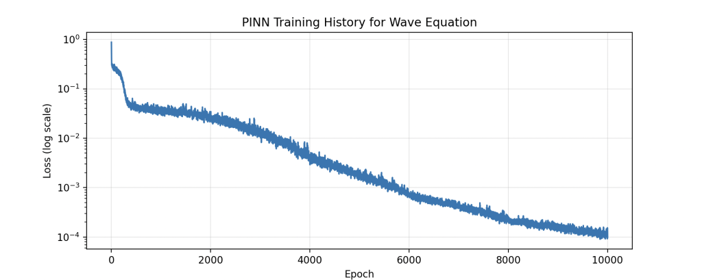
FIG.1. PINN Training History for Wave Equation
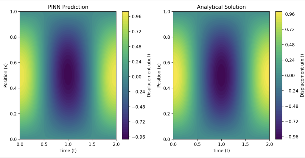
FIG.2. Comparision between prediction result(left) and analytical solution(right)
FIG.2 draws the two-dimensional heat map to show that, with x-axis time increase, different position of the string(y-axis) has different state of displacement, and vibration between positive max value and negative minimum value. And with the comparision between prediction and analytical, we can see that there is no significant error between the two, demonstrating the high accuracy of our model.
We use matplotlib code to generate the vibration demonstration, and in this demonstration, we can see the red dashed line (which indicates the PINN prediction) matches the analytical solution very well, with low absolute error below 0.1 at the same time.
References
[1]吴崇试, 高春媛. 数学物理方法[M]. 北京大学出版社:202408:558
[2]许明. 物理信息神经网络(PINN)求解二阶微分方程及有限元方法对比分析[EB/OL]. (2025-08-24)[2025-11-24]. https://mp.weixin.qq.com/s/mP6xz4KcFB8oHwVSf2mj4A.
Appendix
import torch
import torch.nn as nn
import numpy as np
import matplotlib.pyplot as plt
from matplotlib.animation import FuncAnimation
# 设置随机种子
torch.manual_seed(42)
np.random.seed(42)
# =========================
# 1. 定义问题参数
# =========================
L = 1.0 # 弦的长度 [m]
c = 1.0 # 波速 [m/s]
T_max = 2.0 # 模拟的总时间 [s]
# 定义解析解用于验证
def analytical_solution(x, t):
"""计算一维波动方程的解析解(驻波)"""
return torch.sin(np.pi * x / L) * torch.cos(np.pi * c * t / L)
# =========================
# 2. 定义PINN模型 (输入是x和t两个变量)
# =========================
class WavePINN(nn.Module):
def __init__(self):
super(WavePINN, self).__init__()
self.net = nn.Sequential(
nn.Linear(2, 64), # 输入维度为2: (x, t)
nn.Tanh(),
nn.Linear(64, 64),
nn.Tanh(),
nn.Linear(64, 64),
nn.Tanh(),
nn.Linear(64, 1), # 输出维度为1: u(x,t)
)
def forward(self, x, t):
# 将x和t合并为一个输入张量
inputs = torch.cat([x, t], dim=1)
return self.net(inputs)
# =========================
# 3. 定义残差计算函数 (核心:计算时空导数)
# =========================
def compute_wave_residual(x, t):
"""
计算波动方程的残差: u_tt - c^2 * u_xx = 0
"""
# 设置需要计算梯度
x.requires_grad_(True)
t.requires_grad_(True)
# 网络预测位移u
u = model(x, t)
# 计算一阶偏导
u_t = torch.autograd.grad(u, t, grad_outputs=torch.ones_like(u),
create_graph=True, retain_graph=True)[0]
u_x = torch.autograd.grad(u, x, grad_outputs=torch.ones_like(u),
create_graph=True, retain_graph=True)[0]
# 计算二阶偏导
u_tt = torch.autograd.grad(u_t, t, grad_outputs=torch.ones_like(u_t),
create_graph=True, retain_graph=True)[0]
u_xx = torch.autograd.grad(u_x, x, grad_outputs=torch.ones_like(u_x),
create_graph=True)[0]
# 波动方程残差
residual = u_tt - (c ** 2) * u_xx
return residual
# =========================
# 4. 定义损失函数 (包含方程残差、边界条件和初始条件)
# =========================
def wave_loss_function():
total_loss = 0.0
batch_size = 100 # 每个损失的采样点数量
# 1. 方程残差损失 (在时空域内部采样)
x_domain = torch.rand(batch_size, 1) * L # [0, L]随机采样
t_domain = torch.rand(batch_size, 1) * T_max # [0, T_max]随机采样
residual = compute_wave_residual(x_domain, t_domain)
loss_pde = torch.mean(residual ** 2)
total_loss += loss_pde
# 2. 边界条件损失 (在时间边界上采样)
t_boundary = torch.rand(batch_size, 1) * T_max
# 左边界 (x=0)
u_left = model(torch.zeros_like(t_boundary), t_boundary)
loss_left_bc = torch.mean(u_left ** 2) # u(0,t) = 0
# 右边界 (x=L)
u_right = model(torch.ones_like(t_boundary) * L, t_boundary)
loss_right_bc = torch.mean(u_right ** 2) # u(L,t) = 0
total_loss += loss_left_bc + loss_right_bc
# 3. 初始条件损失 (在空间域上采样,t=0)
x_initial = torch.rand(batch_size, 1) * L
# 初始位移条件
u_initial = model(x_initial, torch.zeros_like(x_initial))
u_initial_true = torch.sin(np.pi * x_initial / L) # u(x,0) = sin(πx/L)
loss_initial_u = torch.mean((u_initial - u_initial_true) ** 2)
# 初始速度条件 (需要计算时间导数)
x_initial.requires_grad_(False) # 临时禁用梯度,因为我们要对t求导
t_initial = torch.zeros_like(x_initial)
t_initial.requires_grad_(True)
u_initial_pred = model(x_initial, t_initial)
u_t_initial = torch.autograd.grad(u_initial_pred, t_initial,
grad_outputs=torch.ones_like(u_initial_pred),
create_graph=True)[0]
loss_initial_ut = torch.mean(u_t_initial ** 2) # u_t(x,0) = 0
total_loss += loss_initial_u + loss_initial_ut
return total_loss
# =========================
# 5. 模型训练
# =========================
model = WavePINN()
optimizer = torch.optim.Adam(model.parameters(), lr=0.001)
scheduler = torch.optim.lr_scheduler.StepLR(optimizer, step_size=2000, gamma=0.5)
epochs = 10000
loss_history = []
print("开始训练波动方程PINN...")
for epoch in range(epochs):
optimizer.zero_grad()
loss = wave_loss_function()
loss.backward()
optimizer.step()
scheduler.step()
loss_history.append(loss.item())
if epoch % 1000 == 0:
print(f'Epoch {epoch}, Loss: {loss.item():.6f}')
print("训练完成!")
# =========================
# 6. 结果可视化与验证
# =========================
# 准备测试数据
x_test = torch.linspace(0, L, 100).view(-1, 1)
t_test = torch.linspace(0, T_max, 50).view(-1, 1)
# 创建网格进行预测
X, T = torch.meshgrid(x_test.squeeze(), t_test.squeeze(), indexing='ij')
x_flat = X.flatten().view(-1, 1)
t_flat = T.flatten().view(-1, 1)
with torch.no_grad():
u_pred = model(x_flat, t_flat)
U_pred = u_pred.view(X.shape).numpy()
u_analytical = analytical_solution(x_flat, t_flat)
U_analytical = u_analytical.view(X.shape).numpy()
X_np = X.numpy()
T_np = T.numpy()
# 绘制时空演化图
plt.figure(figsize=(15, 5))
# 子图1: PINN预测结果
plt.subplot(1, 3, 1)
contour1 = plt.contourf(T_np, X_np, U_pred, levels=50, cmap='viridis')
plt.colorbar(contour1, label='Displacement u(x,t)')
plt.xlabel('Time (t)')
plt.ylabel('Position (x)')
plt.title('PINN Prediction')
# 子图2: 解析解
plt.subplot(1, 3, 2)
contour2 = plt.contourf(T_np, X_np, U_analytical, levels=50, cmap='viridis')
plt.colorbar(contour2, label='Displacement u(x,t)')
plt.xlabel('Time (t)')
plt.ylabel('Position (x)')
plt.title('Analytical Solution')
# 子图3: 绝对误差
plt.subplot(1, 3, 3)
error = np.abs(U_pred - U_analytical)
contour3 = plt.contourf(T_np, X_np, error, levels=50, cmap='hot')
plt.colorbar(contour3, label='Absolute Error')
plt.xlabel('Time (t)')
plt.ylabel('Position (x)')
plt.title('Absolute Error')
plt.tight_layout()
plt.show()
# 绘制损失曲线
plt.figure(figsize=(10, 4))
plt.plot(loss_history)
plt.yscale('log')
plt.xlabel('Epoch')
plt.ylabel('Loss (log scale)')
plt.title('PINN Training History for Wave Equation')
plt.grid(True, alpha=0.3)
plt.show()
# =========================
# 7. 创建动画展示振动过程
# =========================
print("生成振动动画...")
fig, (ax1, ax2) = plt.subplots(2, 1, figsize=(10, 8))
x_plot = x_test.numpy()
def animate(frame):
t_val = frame * T_max / 50
t_vec = torch.ones_like(x_test) * t_val
with torch.no_grad():
u_pred_frame = model(x_test, t_vec).numpy()
u_true_frame = analytical_solution(x_test, t_vec).numpy()
ax1.clear()
ax2.clear()
# 上部:位移对比
ax1.plot(x_plot, u_true_frame, 'k-', linewidth=2, label='Analytical')
ax1.plot(x_plot, u_pred_frame, 'r--', linewidth=2, label='PINN Prediction')
ax1.set_ylabel('Displacement u(x)')
ax1.set_ylim([-1.2, 1.2])
ax1.legend()
ax1.grid(True, alpha=0.3)
ax1.set_title(f'Wave Propagation at t = {t_val:.2f}s')
# 下部:误差
error_frame = np.abs(u_pred_frame - u_true_frame)
ax2.plot(x_plot, error_frame, 'b-', linewidth=1, label='Error')
ax2.set_ylabel('Absolute Error')
ax2.set_ylim([0, 0.1])
ax2.set_xlabel('Position x')
ax2.legend()
ax2.grid(True, alpha=0.3)
return ax1, ax2
# 创建动画
anim = FuncAnimation(fig, animate, frames=50, interval=100, blit=False)
plt.tight_layout()
plt.show()
# 计算整体误差
total_error = np.mean(np.abs(U_pred - U_analytical))
print(f"Mean Absolute Error over entire domain: {total_error:.6f}")